|
||||||||||||||||||||||||||||||||||||||||||||||||||||||||||||||||||||||||||||||||||||||||||||||||||||||||||||||||||||||||||||||||||||||||||||
|
||||||||||||||||||||||||||||||||||||||||||||||||||||||||||||||||||||||||||||||||||||||||||||||||||||||||||||||||||||||||||||||||||||||||||||
| ||||||||||||||||||||||||||||||||||||||||||||||||||||||||||||||||||||||||||||||||||||||||||||||||||||||||||||||||||||||||||||||||||||||||||||
PMML 4.4.1 - Bayesian Network ModelsA Bayesian Network (BN) is a directed acyclic graphical model representing a joint probability distribution over a set of random variables. The graphical model of a BN consists of nodes and arcs, where nodes represent the random variables (continuous and/or categorical) and arcs represent the causal dependence relationships between several random variables. Given new data on any of the random variables, the Bayesian network model can be used to infer all the remaining random variables. Thus, a Bayesian network can be used for both probabilistic regression and classification. If X={X1,X2...,Xn} is a set of n random variables, then a Bayesian network B, over these random variables can be represented as PrB(X) =
n
∏
i=1
PrB(Xi | ΠXi)
where ΠXi represents the set of parent nodes of Xi and PrB(Xi | ΠXi) represents the conditional probability distribution of Xi, given its parent nodes. If Xi has no parent nodes, then PrB(Xi | ΠXi) represents the marginal probability distribution of Xi. Variables with no parent nodes are often referred to as root variables. Note that, as mentioned above, the variables in a Bayesian network can be categorical or continuous. For continuous variables, conditional or marginal probability distributions are defined whereas for categorical variables, conditional or marginal probability tables are defined. Let Nobs represent the subset of variables about which new data (D) is available. This new information can be used along with the available Bayesian network model to estimate the posterior probabilities for the variables for which there is no new data (unobserved variables), represented as Nobs, using the Bayes theorem as Pr(Nobs | Nobs = D) ∝ Pr(Nobs = D | Nobs ) Pr(Nobs)
where Pr(Nobs) and Pr(Nobs | Nobs = D) represent the prior and posterior distributions of the unobserved variables, respectively. Pr(Nobs = D | Nobs ) represents the likelihood of observing the data (D) conditioned on the unobserved variables. Exact computation of the posterior distributions can become computationally expensive; in such cases, approximate techniques such as Markov Chain Monte Carlo (MCMC) methods, Approximate Bayesian Computation (ABC) can be used to obtain the posterior distributions. Representation of a Bayesian network in a PMML format requires the storage of the following information
Bayesian Network Model schema <xs:element name="BayesianNetworkModel"> <xs:complexType> <xs:sequence> <xs:element ref="Extension" minOccurs="0" maxOccurs="unbounded"/> <xs:element ref="MiningSchema"/> <xs:element ref="Output" minOccurs="0"/> <xs:element ref="ModelStats" minOccurs="0"/> <xs:element ref="ModelExplanation" minOccurs="0"/> <xs:element ref="Targets" minOccurs="0"/> <xs:element ref="LocalTransformations" minOccurs="0"/> <xs:element ref="BayesianNetworkNodes" minOccurs="1"/> <xs:element ref="ModelVerification" minOccurs="0"/> <xs:element ref="Extension" minOccurs="0" maxOccurs="unbounded"/> </xs:sequence> <xs:attribute name="modelName" type="xs:string"/> <xs:attribute name="functionName" type="MINING-FUNCTION" use="required"/> <xs:attribute name="algorithmName" type="xs:string"/> <xs:attribute name="modelType" type="BN-TYPE" default="General"/> <xs:attribute name="inferenceMethod" type="INFERENCE-TYPE" default="Other"/> <xs:attribute name="isScorable" type="xs:boolean" default="true"/> </xs:complexType> </xs:element> <xs:simpleType name="BN-TYPE"> <xs:restriction base="xs:string"> <xs:enumeration value="General"/> <xs:enumeration value="TAN"/> <xs:enumeration value="Markov-blanket"/> </xs:restriction> </xs:simpleType> <xs:simpleType name="INFERENCE-TYPE"> <xs:restriction base="xs:string"> <xs:enumeration value="Other"/> <xs:enumeration value="MCMC"/> <xs:enumeration value="Exact"/> </xs:restriction> </xs:simpleType> modelName and algorithmName can have arbitrary strings describing the specific model and algorithm. functionName can only be classification or regression. modelType is an optional enumerated attribute that can be
General, TAN or Markov-blanket. This facilitates the selection of more efficient inference algorithms when possible. inferenceMethod: This optional attribute specifies the suggested inference method for this model. The allowed values are
MCMC, Exact, and Other. isScorable: This attribute indicates if the model is valid for scoring. If this attribute is true or if it is missing, then the model should be processed normally. However, if the attribute is false, then the model producer has indicated that this model is intended for information purposes only and should not be used to generate results. In order to be valid PMML, all required elements and attributes must be present, even for non-scoring models. For more details, see General Structure. Node Types The Bayesian Network can have two types of nodes - discrete and continuous. Discrete nodes have a limited set of possible values. They have value probabilities if they are not conditioned on other nodes, or have a conditional probability table if they are conditioned on other nodes. The sum of the value probabilities must equal 1. The optional attribute count can be used to track the total number of cases used to generate the probabilities. <xs:element name="BayesianNetworkNodes"> <xs:complexType> <xs:sequence> <xs:element ref="Extension" minOccurs="0" maxOccurs="unbounded"/> <xs:choice maxOccurs="unbounded"> <xs:element ref="DiscreteNode"/> <xs:element ref="ContinuousNode"/> </xs:choice> </xs:sequence> </xs:complexType> </xs:element> <xs:element name="DiscreteNode"> <xs:complexType> <xs:sequence> <xs:element ref="Extension" minOccurs="0" maxOccurs="unbounded"/> <xs:element ref="DerivedField" minOccurs="0" maxOccurs="unbounded"/> <xs:choice maxOccurs="unbounded"> <xs:element ref="DiscreteConditionalProbability"/> <xs:element ref="ValueProbability" maxOccurs="unbounded"/> </xs:choice> </xs:sequence> <xs:attribute name="name" type="FIELD-NAME" use="required"/> <xs:attribute name="count" type="REAL-NUMBER" use="optional"/> </xs:complexType> </xs:element> <xs:element name="ContinuousNode"> <xs:complexType> <xs:sequence> <xs:element ref="Extension" minOccurs="0" maxOccurs="unbounded"/> <xs:element ref="DerivedField" minOccurs="0" maxOccurs="unbounded"/> <xs:choice maxOccurs="unbounded"> <xs:element ref="ContinuousConditionalProbability"/> <xs:element ref="ContinuousDistribution" maxOccurs="unbounded"/> </xs:choice> </xs:sequence> <xs:attribute name="name" type="FIELD-NAME" use="required"/> <xs:attribute name="count" type="REAL-NUMBER" use="optional"/> </xs:complexType> </xs:element> Conditional Probabilities When a node is conditioned upon its parent nodes in the network, its value is given by a conditional probability table that specifies the value probabilities for different combinations of values of the parent nodes. DiscreteConditionalProbability elements are used to specify conditional probabilities for discrete nodes. The DiscreteConditionalProbability element contains a ParentValue element and a ValueProbability element, to specify the value probability for each value of the parent node. The schema for representing discrete conditional probability tables is given below. <xs:element name="DiscreteConditionalProbability"> <xs:complexType> <xs:sequence> <xs:element ref="Extension" minOccurs="0" maxOccurs="unbounded"/> <xs:element ref="ParentValue" minOccurs="1" maxOccurs="unbounded"/> <xs:element ref="ValueProbability" minOccurs="1" maxOccurs="unbounded"/> </xs:sequence> <xs:attribute name="count" type="REAL-NUMBER" use="optional"/> </xs:complexType> </xs:element> <xs:element name="ParentValue"> <xs:complexType> <xs:sequence> <xs:element ref="Extension" minOccurs="0" maxOccurs="unbounded"/> </xs:sequence> <xs:attribute name="parent" type="FIELD-NAME" use="required"/> <xs:attribute name="value" type="xs:string" use="required"/> </xs:complexType> </xs:element> <xs:element name="ValueProbability"> <xs:complexType> <xs:sequence> <xs:element ref="Extension" minOccurs="0" maxOccurs="unbounded"/> </xs:sequence> <xs:attribute name="value" type="xs:string" use="required"/> <xs:attribute name="probability" type="PROB-NUMBER" use="required"/> </xs:complexType> </xs:element> For continuous nodes, the value is represented by a continuous distribution. The schema allows the parameters of the distribution to be represented by expressions, allowing them to be functions of other node values. ContinuousConditionalProbability elements are used to represent the conditional probability of continuous nodes. In this case, ParentValue is optional, and only needed to specify conditional probabilities for discrete values of parent nodes. For continuous parent nodes, the conditional probabilities are represented by incorporating the parent value in the distribution parameters. The schema for representing continuous distributions and conditional probability tables is given below. <xs:element name="ContinuousConditionalProbability"> <xs:complexType> <xs:sequence> <xs:element ref="Extension" minOccurs="0" maxOccurs="unbounded"/> <xs:element ref="ParentValue" minOccurs="0" maxOccurs="unbounded"/> <xs:element ref="ContinuousDistribution" minOccurs="1" maxOccurs="unbounded"/> </xs:sequence> <xs:attribute name="count" type="REAL-NUMBER" use="optional"/> </xs:complexType> </xs:element> <xs:element name="ContinuousDistribution"> <xs:complexType> <xs:sequence> <xs:element ref="Extension" minOccurs="0" maxOccurs="unbounded"/> <xs:choice> <xs:element ref="TriangularDistributionForBN"/> <xs:element ref="NormalDistributionForBN"/> <xs:element ref="LognormalDistributionForBN"/> <xs:element ref="UniformDistributionForBN"/> </xs:choice> </xs:sequence> </xs:complexType> </xs:element> <xs:element name="TriangularDistributionForBN"> <xs:complexType> <xs:sequence> <xs:element ref="Extension" minOccurs="0" maxOccurs="unbounded"/> <xs:element ref="Mean" minOccurs="1" maxOccurs="1"/> <xs:element ref="Lower" minOccurs="1" maxOccurs="1"/> <xs:element ref="Upper" minOccurs="1" maxOccurs="1"/> </xs:sequence> </xs:complexType> </xs:element> <xs:element name="NormalDistributionForBN"> <xs:complexType> <xs:sequence> <xs:element ref="Extension" minOccurs="0" maxOccurs="unbounded"/> <xs:element ref="Mean" minOccurs="1" maxOccurs="1"/> <xs:element ref="Variance" minOccurs="1" maxOccurs="1"/> </xs:sequence> </xs:complexType> </xs:element> <xs:element name="LognormalDistributionForBN"> <xs:complexType> <xs:sequence> <xs:element ref="Extension" minOccurs="0" maxOccurs="unbounded"/> <xs:element ref="Mean" minOccurs="1" maxOccurs="1"/> <xs:element ref="Variance" minOccurs="1" maxOccurs="1"/> </xs:sequence> </xs:complexType> </xs:element> <xs:element name="UniformDistributionForBN"> <xs:complexType> <xs:sequence> <xs:element ref="Extension" minOccurs="0" maxOccurs="unbounded"/> <xs:element ref="Lower" minOccurs="1" maxOccurs="1"/> <xs:element ref="Upper" minOccurs="1" maxOccurs="1"/> </xs:sequence> </xs:complexType> </xs:element> <xs:element name="Mean"> <xs:complexType> <xs:sequence> <xs:element ref="Extension" minOccurs="0" maxOccurs="unbounded"/> <xs:group ref="EXPRESSION"/> </xs:sequence> </xs:complexType> </xs:element> <xs:element name="Lower"> <xs:complexType> <xs:sequence> <xs:element ref="Extension" minOccurs="0" maxOccurs="unbounded"/> <xs:group ref="EXPRESSION"/> </xs:sequence> </xs:complexType> </xs:element> <xs:element name="Upper"> <xs:complexType> <xs:sequence> <xs:element ref="Extension" minOccurs="0" maxOccurs="unbounded"/> <xs:group ref="EXPRESSION"/> </xs:sequence> </xs:complexType> </xs:element> <xs:element name="Variance"> <xs:complexType> <xs:sequence> <xs:element ref="Extension" minOccurs="0" maxOccurs="unbounded"/> <xs:group ref="EXPRESSION"/> </xs:sequence> </xs:complexType> </xs:element> Scoring Procedure and Examples Scoring for Bayesian Networks (called inference) is performed by computing the conditional probabilities of the variables in the network after fixing the known variables. In many cases, this is a hard problem for general Bayesian networks. In such cases, approximate inference methods based on statistical sampling are used. Here, we present two examples: one exact inference example based on analytically computing the conditional probabilities, and one approximate inference example based on Markov Chain Monte Carlo (MCMC) methods. First, a scoring example with PMML/BN is provided here for illustration. An example BN is shown below, along with the prior probabilities for the nodes. The BN in the figure below has a combination of continuous and discrete nodes. The prior probabilities and discrete and continuous conditional probability tables are listed below. In the Bayesian network shown below, let us say that new observations on two variables D4, C4 are available, for example, D4 = 0 and C4 = 7. This new information will be used to estimate unobserved variables, i.e., D1, D2, D3, C1, C2, and C3. 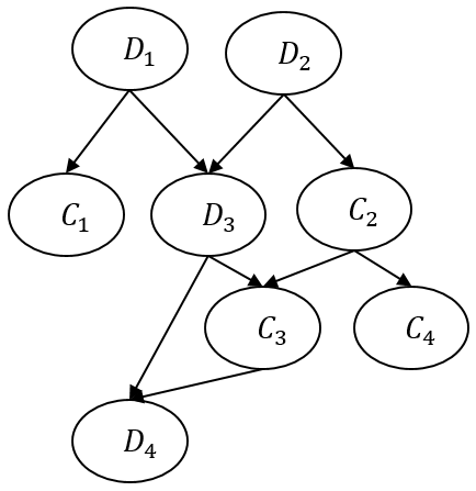
The PMML file for the BN example above is shown here: <PMML xmlns="https://www.dmg.org/PMML-4_4" version="4.4">
<Header copyright="DMG.org"/>
<DataDictionary numberOfFields="8">
<DataField dataType="double" name="C1" optype="continuous"/>
<DataField dataType="double" name="C2" optype="continuous"/>
<DataField dataType="double" name="C3" optype="continuous"/>
<DataField dataType="double" name="C4" optype="continuous"/>
<DataField dataType="string" name="D1" optype="categorical">
<Value value="0"/>
<Value value="1"/>
</DataField>
<DataField dataType="string" name="D2" optype="categorical">
<Value value="0"/>
<Value value="1"/>
<Value value="2"/>
</DataField>
<DataField dataType="string" name="D3" optype="categorical">
<Value value="0"/>
<Value value="1"/>
</DataField>
<DataField dataType="string" name="D4" optype="categorical">
<Value value="0"/>
<Value value="1"/>
</DataField>
</DataDictionary>
<BayesianNetworkModel modelName="BN Example" functionName="regression" inferenceMethod="MCMC">
<MiningSchema>
<MiningField name="D4" usageType="active"/>
<MiningField name="C4" usageType="active"/>
<MiningField name="D1" usageType="target"/>
<MiningField name="D2" usageType="target"/>
<MiningField name="D3" usageType="target"/>
<MiningField name="C1" usageType="target"/>
<MiningField name="C2" usageType="target"/>
<MiningField name="C3" usageType="target"/>
</MiningSchema>
<BayesianNetworkNodes>
<!-- -->
<DiscreteNode name="D1">
<ValueProbability value="0" probability="0.3"/>
<ValueProbability value="1" probability="0.7"/>
</DiscreteNode>
<!-- -->
<DiscreteNode name="D2">
<ValueProbability value="0" probability="0.6"/>
<ValueProbability value="1" probability="0.3"/>
<ValueProbability value="2" probability="0.1"/>
</DiscreteNode>
<!-- -->
<DiscreteNode name="D3">
<DiscreteConditionalProbability>
<ParentValue parent="D1" value="0"/>
<ParentValue parent="D2" value="0"/>
<ValueProbability value="0" probability="0.1"/>
<ValueProbability value="1" probability="0.9"/>
</DiscreteConditionalProbability>
<DiscreteConditionalProbability>
<ParentValue parent="D1" value="0"/>
<ParentValue parent="D2" value="1"/>
<ValueProbability value="0" probability="0.3"/>
<ValueProbability value="1" probability="0.7"/>
</DiscreteConditionalProbability>
<DiscreteConditionalProbability>
<ParentValue parent="D1" value="0"/>
<ParentValue parent="D2" value="2"/>
<ValueProbability value="0" probability="0.4"/>
<ValueProbability value="1" probability="0.6"/>
</DiscreteConditionalProbability>
<DiscreteConditionalProbability>
<ParentValue parent="D1" value="1"/>
<ParentValue parent="D2" value="0"/>
<ValueProbability value="0" probability="0.6"/>
<ValueProbability value="1" probability="0.4"/>
</DiscreteConditionalProbability>
<DiscreteConditionalProbability>
<ParentValue parent="D1" value="1"/>
<ParentValue parent="D2" value="1"/>
<ValueProbability value="0" probability="0.8"/>
<ValueProbability value="1" probability="0.2"/>
</DiscreteConditionalProbability>
<DiscreteConditionalProbability>
<ParentValue parent="D1" value="1"/>
<ParentValue parent="D2" value="2"/>
<ValueProbability value="0" probability="0.9"/>
<ValueProbability value="1" probability="0.1"/>
</DiscreteConditionalProbability>
</DiscreteNode>
<!-- -->
<ContinuousNode name="C1">
<ContinuousConditionalProbability>
<ParentValue parent="D1" value="0"/>
<ContinuousDistribution>
<NormalDistributionForBN>
<Mean>
<Constant dataType="double">10</Constant>
</Mean>
<Variance>
<Constant dataType="double">2</Constant>
</Variance>
</NormalDistributionForBN>
</ContinuousDistribution>
</ContinuousConditionalProbability>
<ContinuousConditionalProbability>
<ParentValue parent="D1" value="1"/>
<ContinuousDistribution>
<NormalDistributionForBN>
<Mean>
<Constant dataType="double">14</Constant>
</Mean>
<Variance>
<Constant dataType="double">2</Constant>
</Variance>
</NormalDistributionForBN>
</ContinuousDistribution>
</ContinuousConditionalProbability>
</ContinuousNode>
<!-- -->
<ContinuousNode name="C2">
<ContinuousConditionalProbability>
<ParentValue parent="D2" value="0"/>
<ContinuousDistribution>
<NormalDistributionForBN>
<Mean>
<Constant dataType="double">6</Constant>
</Mean>
<Variance>
<Constant dataType="double">1</Constant>
</Variance>
</NormalDistributionForBN>
</ContinuousDistribution>
</ContinuousConditionalProbability>
<ContinuousConditionalProbability>
<ParentValue parent="D2" value="1"/>
<ContinuousDistribution>
<NormalDistributionForBN>
<Mean>
<Constant dataType="double">8</Constant>
</Mean>
<Variance>
<Constant dataType="double">1</Constant>
</Variance>
</NormalDistributionForBN>
</ContinuousDistribution>
</ContinuousConditionalProbability>
<ContinuousConditionalProbability>
<ParentValue parent="D2" value="2"/>
<ContinuousDistribution>
<NormalDistributionForBN>
<Mean>
<Constant dataType="double">14</Constant>
</Mean>
<Variance>
<Constant dataType="double">1</Constant>
</Variance>
</NormalDistributionForBN>
</ContinuousDistribution>
</ContinuousConditionalProbability>
</ContinuousNode>
<!-- -->
<ContinuousNode name="C4">
<ContinuousConditionalProbability>
<ContinuousDistribution>
<NormalDistributionForBN>
<Mean>
<Apply function="+">
<Apply function="*">
<Constant dataType="double">0.1</Constant>
<Apply function="pow">
<FieldRef field="C2"/>
<Constant dataType="integer">2</Constant>
</Apply>
</Apply>
<Apply function="+">
<Apply function="*">
<Constant dataType="double">0.6</Constant>
<FieldRef field="C2"/>
</Apply>
<Constant dataType="integer">1</Constant>
</Apply>
</Apply>
</Mean>
<Variance>
<Constant dataType="double">2</Constant>
</Variance>
</NormalDistributionForBN>
</ContinuousDistribution>
</ContinuousConditionalProbability>
</ContinuousNode>
<!-- -->
<ContinuousNode name="C3">
<ContinuousConditionalProbability>
<ParentValue parent="D3" value="0"/>
<ContinuousDistribution>
<NormalDistributionForBN>
<Mean>
<Apply function="*">
<Constant dataType="double">0.15</Constant>
<Apply function="pow">
<FieldRef field="C2"/>
<Constant dataType="integer">2</Constant>
</Apply>
</Apply>
</Mean>
<Variance>
<Constant dataType="double">2</Constant>
</Variance>
</NormalDistributionForBN>
</ContinuousDistribution>
</ContinuousConditionalProbability>
<ContinuousConditionalProbability>
<ParentValue parent="D3" value="1"/>
<ContinuousDistribution>
<NormalDistributionForBN>
<Mean>
<Apply function="*">
<Constant dataType="double">1.5</Constant>
<FieldRef field="C2"/>
</Apply>
</Mean>
<Variance>
<Constant dataType="double">1</Constant>
</Variance>
</NormalDistributionForBN>
</ContinuousDistribution>
</ContinuousConditionalProbability>
</ContinuousNode>
<!-- -->
<DiscreteNode name="D4">
<DerivedField name="C3_Discretized" optype="categorical" dataType="string">
<Discretize field="C3">
<DiscretizeBin binValue="0">
<Interval closure="openClosed" rightMargin="9"/>
</DiscretizeBin>
<DiscretizeBin binValue="1">
<Interval closure="openClosed" leftMargin="9" rightMargin="11"/>
</DiscretizeBin>
<DiscretizeBin binValue="2">
<Interval closure="openOpen" leftMargin="11"/>
</DiscretizeBin>
</Discretize>
</DerivedField>
<DiscreteConditionalProbability>
<ParentValue parent="D3" value="0"/>
<ParentValue parent="C3_Discretized" value="0"/>
<ValueProbability value="0" probability="0.4"/>
<ValueProbability value="1" probability="0.6"/>
</DiscreteConditionalProbability>
<DiscreteConditionalProbability>
<ParentValue parent="D3" value="0"/>
<ParentValue parent="C3_Discretized" value="1"/>
<ValueProbability value="0" probability="0.3"/>
<ValueProbability value="1" probability="0.7"/>
</DiscreteConditionalProbability>
<DiscreteConditionalProbability>
<ParentValue parent="D3" value="0"/>
<ParentValue parent="C3_Discretized" value="2"/>
<ValueProbability value="0" probability="0.6"/>
<ValueProbability value="1" probability="0.4"/>
</DiscreteConditionalProbability>
<DiscreteConditionalProbability>
<ParentValue parent="D3" value="1"/>
<ParentValue parent="C3_Discretized" value="0"/>
<ValueProbability value="0" probability="0.4"/>
<ValueProbability value="1" probability="0.6"/>
</DiscreteConditionalProbability>
<DiscreteConditionalProbability>
<ParentValue parent="D3" value="1"/>
<ParentValue parent="C3_Discretized" value="1"/>
<ValueProbability value="0" probability="0.1"/>
<ValueProbability value="1" probability="0.9"/>
</DiscreteConditionalProbability>
<DiscreteConditionalProbability>
<ParentValue parent="D3" value="1"/>
<ParentValue parent="C3_Discretized" value="2"/>
<ValueProbability value="0" probability="0.3"/>
<ValueProbability value="1" probability="0.7"/>
</DiscreteConditionalProbability>
</DiscreteNode>
</BayesianNetworkNodes>
</BayesianNetworkModel>
</PMML>
Let Nobs, Nobs and D denote the set of observed, unobserved variables and available data, respectively. Using the Bayes theorem, the updated (posterior) probability distributions of the unobserved variables can be estimated as Pr(Nobs | Nobs = D) ∝ Pr(Nobs = D | Nobs) Pr(Nobs) Solving the above expression can be computationally expensive; therefore, approximate methods such as Markov Chain Monte Carlo (MCMC) methods are used to obtain posterior distributions of unknown variables. The MCMC methods represent a class of algorithms for probabilistic inference in stochastic models such as Bayesian networks. Some commonly used MCMC algorithms are:
The idea of selecting a statistical sample to approximate a hard combinatorial problem by a much simpler problem is at the heart of modern Monte Carlo simulation. There are several high-dimensional problems, such as computing the volume of a convex body in d dimensions, for which Markov Chain Monte Carlo (MCMC) simulation, a large class of sampling algorithms, is the only known general approach for providing a solution within a reasonable time (polynomial in d) (Andrieu et al., 2003). When performing Bayesian inference, we aim to compute and use the full posterior joint distribution over a set of random variables. Unfortunately, this often requires calculating intractable integrals. In such cases, we may give up on solving the analytical equations, and proceed with sampling techniques based upon MCMC methods. When using MCMC methods, we estimate the posterior distribution and the intractable integrals using simulated samples from the posterior distribution. Metropolis-Hastings algorithms are particular instances of a large family of MCMC algorithms, which also includes the Boltzmann algorithm (Hastings, 1970). The Metropolis-Hastings (MH) algorithm simulates samples from a probability distribution by making use of the full joint density function and (independent) proposal distributions for each of the variables of interest. The algorithm below provides the details of a generic MH algorithm (Yildirim, 2012). 
In this example, we used Metropolis-Hastings algorithm for inference. Here, let P(x) be the true posterior distribution of parameters which need to be determined. Computation of P(x) analytically is NP hard, therefore, we use approximate techniques (MCMC) to generate some samples from P(x). In Metropolis-Hastings algorithm, we generate samples from a different distribution(called proposal distribution), represented as Q(x), and check their ability to be in the true posterior distribution P(x). The rest of the algorithm is as follows:
The MCMC chain converges after some initial samples. MCMC chain is said to be converged if there is no significant change in the posterior distributions when the length of the chain is increased. Consider the figure below of a sample MCMC chain, with three segments of the chain highlighted after initial burn-in. We can construct and compare posterior distributions using the first and second sections. If there is no significant difference, we can assume the chain is converged. If there is significant variation, we can go on to the third section and construct the posterior distribution. Similarly, if there is no change between second and third sections, we can stop the chain else we can go on to the fourth section (not shown). The samples from the converged part of the chain can be used to construct approximations to the true posterior distributions. 
Using the MCMC algorithms, samples from the joint posterior distribution can be obtained and hence marginal distributions can be constructed. For categorical variables, D1, D2, and D3, the change in the probabilities of each of the states due to the new information is given below.
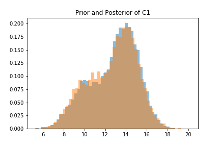
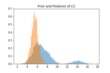
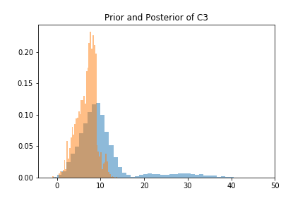
Similarly, for continuous variables C1, C2, and C3, their entire prior and posterior probability distributions can be constructed. Along the distributions, their mean’s and variance’s, shown below, are obtained.
Exact Inference Example Here, we provide an additional, exact inference example. A BN is shown below, along with the conditional probability tables. 
The PMML file for the BN example above are shown here: <PMML xmlns="https://www.dmg.org/PMML-4_4" version="4.4">
<Header copyright="DMG.org"/>
<DataDictionary numberOfFields="3">
<DataField dataType="string" name="A" optype="categorical">
<Value value="0"/>
<Value value="1"/>
</DataField>
<DataField dataType="string" name="B" optype="categorical">
<Value value="0"/>
<Value value="1"/>
</DataField>
<DataField dataType="string" name="C" optype="categorical">
<Value value="0"/>
<Value value="1"/>
<Value value="2"/>
</DataField>
</DataDictionary>
<BayesianNetworkModel modelName="BN Example" functionName="regression" inferenceMethod="Exact">
<MiningSchema>
<MiningField name="A" usageType="target"/>
<MiningField name="B" usageType="target"/>
<MiningField name="C" usageType="active"/>
</MiningSchema>
<BayesianNetworkNodes>
<DiscreteNode name="A">
<ValueProbability value="0" probability="0.4"/>
<ValueProbability value="1" probability="0.6"/>
</DiscreteNode>
<DiscreteNode name="B">
<ValueProbability value="0" probability="0.7"/>
<ValueProbability value="1" probability="0.3"/>
</DiscreteNode>
<DiscreteNode name="C">
<DiscreteConditionalProbability>
<ParentValue parent="A" value="0"/>
<ParentValue parent="B" value="0"/>
<ValueProbability value="0" probability="0.7"/>
<ValueProbability value="1" probability="0.2"/>
<ValueProbability value="2" probability="0.1"/>
</DiscreteConditionalProbability>
<DiscreteConditionalProbability>
<ParentValue parent="A" value="0"/>
<ParentValue parent="B" value="1"/>
<ValueProbability value="0" probability="0.6"/>
<ValueProbability value="1" probability="0.2"/>
<ValueProbability value="2" probability="0.2"/>
</DiscreteConditionalProbability>
<DiscreteConditionalProbability>
<ParentValue parent="A" value="1"/>
<ParentValue parent="B" value="0"/>
<ValueProbability value="0" probability="0.4"/>
<ValueProbability value="1" probability="0.3"/>
<ValueProbability value="2" probability="0.3"/>
</DiscreteConditionalProbability>
<DiscreteConditionalProbability>
<ParentValue parent="A" value="1"/>
<ParentValue parent="B" value="1"/>
<ValueProbability value="0" probability="0.3"/>
<ValueProbability value="1" probability="0.3"/>
<ValueProbability value="2" probability="0.4"/>
</DiscreteConditionalProbability>
</DiscreteNode>
</BayesianNetworkNodes>
</BayesianNetworkModel>
</PMML>
Suppose the new observation (input) is C = 2. We must find the posterior distributions of A, B. According to the Bayes theorem: Pr(A, B|C=2) = Pr(C=2|A,B)Pr(A,B) / Pr(C=2) Pr(A,B|C=2) = k*Pr(C=2|A,B)Pr(A,B), where the constant k = 1 / Pr(C=2) Pr(A,B|C=2) requires computation of Pr(A=0,B=0|C=2), Pr(A=1,B=0|C=2), Pr(A=0,B=1|C=2), and Pr(A=1,B=1|C=2), since A, B are discrete variables with values 0, 1. Pr(A=0,B=0|C=2) = Pr(C=2|A=0,B=0)Pr(A=0,B=0) = k*0.1*0.4*0.7 = 0.028*k Pr(A=0,B=1|C=2) = Pr(C=2|A=0,B=1)Pr(A=0,B=1) = k*0.2*0.4*0.3 = 0.024*k Pr(A=1,B=0|C=2) = Pr(C=2|A=1,B=0)Pr(A=1,B=0) = k*0.3*0.6*0.7 = 0.126*k Pr(A=1,B=1|C=2) = Pr(C=2|A=1,B=1)Pr(A=1,B=1) = k*0.4*0.6*0.3 = 0.072*k The sum of all probability values should be equal to 1: Pr(A=0,B=0|C=2) = 0.028*4 = 0.112 Pr(A=0,B=1|C=2) = 0.024*4 = 0.096 Pr(A=1,B=0|C=2) = 0.126*4 = 0.504 Pr(A=1,B=1|C=2) = 0.028*4 = 0.288 Posterior distribution of A: Posterior distribution of B: References: Hastings, W. Keith. "Monte Carlo sampling methods using Markov chains and their applications." Biometrika 57.1 (1970): 97-109. Andrieu, Christophe, et al. "An introduction to MCMC for machine learning." Machine learning 50.1-2 (2003): 5-43. Yildirim, Ilker. "Bayesian Inference: Metropolis-Hastings Sampling." Dept. of Brain and Cognitive Sciences, Univ. of Rochester, Rochester, NY (2012). |
||||||||||||||||||||||||||||||||||||||||||||||||||||||||||||||||||||||||||||||||||||||||||||||||||||||||||||||||||||||||||||||||||||||||||||
|