PMML 4.0 - Model Explanation
This document gives an overview of components that can hold further information
to explain PMML models. This can be done by, but is not limited to, visualizing the respective information.
The following elements can be used:
While univariate statistics and partitions are included in specific parts of the models, all the remaining elements are
combined into a single element
ModelExplanation.
  <xs:element name="ModelExplanation">
    <xs:complexType>
      <xs:sequence>
        <xs:element ref="Extension" minOccurs="0" maxOccurs="unbounded"/>
          <xs:choice>
            <xs:element ref="PredictiveModelQuality" minOccurs="0" maxOccurs="unbounded"/>
            <xs:element ref="ClusteringModelQuality" minOccurs="0" maxOccurs="unbounded"/>
          </xs:choice>
        <xs:element ref="Correlations" minOccurs="0"/>
      </xs:sequence>
    </xs:complexType>
  </xs:element>
|
To provide univariate statistics for
MiningFields, use
UnivariateStats in the
ModelStats
element as defined in the
statistics section.
See further information there.
Partition elements are defined in the
statistics section.
They can be used to provide statistics for a subset of records defined by the context in which the
Partition element appears.
For instance, a
Partition in a
Cluster element in a
cluster model provides statistics for
all records that belong to that cluster.
A
Partition element inside a
Node element in a
tree model gives statistics on the value distributions of
the subset of records that belong to that
Node. Likewise, a
Partition element in a
TargetValue
gives details on the distributions of the records for which the model predicted the respective
TargetValue.
The
PredictiveModelQuality
element is a wrapper around various elements used to illustrate the
quality of a predictive model. Since it is possible to recalculate model quality information for any given dataset that matches
the fields specified in the
MiningSchema, it also carries information on what dataset the quality information was collected.
  <xs:element name="PredictiveModelQuality">
    <xs:complexType>
      <xs:sequence>
        <xs:element ref="Extension" minOccurs="0" maxOccurs="unbounded"/>
        <xs:element ref="ConfusionMatrix" minOccurs="0"/>
        <xs:element ref="LiftData" minOccurs="0"/>
        <xs:element ref="ROC" minOccurs="0"/>
      </xs:sequence>
      <xs:attribute name="targetField" type="xs:string" use="required"/>
      <xs:attribute name="dataName" type="xs:string" use="optional"/>
      <xs:attribute name="dataUsage" default="training">
        <xs:simpleType>
          <xs:restriction base="xs:string">
            <xs:enumeration value="training"/>
            <xs:enumeration value="test"/>
            <xs:enumeration value="validation"/>
          </xs:restriction>
        </xs:simpleType>
      </xs:attribute>
      <xs:attribute name="meanError" type="NUMBER" use="optional"/>
      <xs:attribute name="meanAbsoluteError" type="NUMBER" use="optional"/>
      <xs:attribute name="meanSquaredError" type="NUMBER" use="optional"/>
      <xs:attribute name="r-squared" type="NUMBER" use="optional"/>
    </xs:complexType>
  </xs:element>
|
See the successive sections for descriptions on ConfusionMatrix and LiftData.
Attribute description:
- targetField: Specifies the field that the model quality information refers to.
Useful in case a model has multiple predicted fields.
- dataName: The name of the dataset where the model quality information was collected on.
- dataUsage: Specifies the phase in which the model quality information was collected.
training refers to the initial model building phase.
validation data are used during model building for tasks other than
model optimization. Such tasks include the computation of algorithm termination conditions.
test is the application of the model to data different from the training data
after the model has been built.
- meanError: The mean of the predictive errors for the data set.
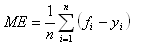
- meanAbsoluteError: The mean of the absolute predictive errors for the data set.
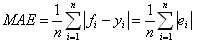
where ei = fi - yi, fi is the prediction and
yi is the true value.
If present, record weighting factors are considered in calculating MAE.
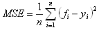
- meanSquaredError: The mean of the squared errors for the data set.
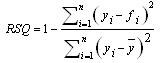
- r-squared: The fraction of the target variation that is accounted for by the model.
Example
  ...
  <ModelQuality targetField="salary" dataName="MyData" dataUsage="training"
                meanError="0.01" meanAbsoluteError="123.4" meanSquaredError="234567.8">
  ...
  </ModelQuality>
  ...
|
In this example, the model quality information for the field salary was gathered
during training on a dataset named MyData.
The
ClusteringModelQuality element is a wrapper around various elements used to illustrate
the quality of a clustering model.
  <xs:element name="ClusteringModelQuality">
    <xs:complexType>
      <xs:attribute name="dataName" type="xs:string" use="optional"/>
      <xs:attribute name="SSE" type="NUMBER" use="optional"/>
      <xs:attribute name="SSB" type="NUMBER" use="optional"/>
    </xs:complexType>
  </xs:element>
|
Attribute description:
- dataName: The name of the dataset where the model quality information was collected on.
- SSE: SSE is a prototype-based cohesion measure where the squared Euclidean distance is used. It is define as:
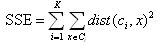
where x is a case belonging to cluster Ci,and ci is the centroid of cluster
Ci, K is the number of clusters.
- SSB: SSB is a prototype-based separation measure where the squared Euclidean distance is used. It is defined as:
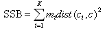
where c is the overall mean and mi is the size of cluster Ci.
Note that SSE and SSB will make sense only when all the inputs are numeric or have been normalized.
Gains and Lift charts are a popular method to display the quality of a predictive data mining model. Regression models have
a single Gainschart for the whole model, classification models can have one for each class label.
The data for a Gains chart is calculated in the following ways:
- For classification models, all predictions are ordered by descending confidence for a specific class label.
- For regression models, all predicted values are ordered by descending magnitude.
The data is then split up into suitable segments of records. The number of segments is up to the user.
The necessary data for Gains and Lift charts is provided in a
LiftData element. It is provided by record counts and
- in case of classification models: The number of records for which the actual value of the predicted field
is the class label in question.
- in case of regression models: The aggregate of the actual values corresponding to the predictions of the interval.
This is essentially a lift representation of the data. The Gains chart can be derived by aggregating the respective value counts.
  <xs:element name="LiftData">
    <xs:complexType>
      <xs:sequence>
        <xs:element ref="Extension" minOccurs="0" maxOccurs="unbounded"/>
        <xs:element ref="ModelLiftGraph"/>
        <xs:element ref="OptimumLiftGraph" minOccurs="0"/>
        <xs:element ref="RandomLiftGraph" minOccurs="0"/>
      </xs:sequence>
      <xs:attribute name="targetFieldValue" type="xs:string"/>
      <xs:attribute name="targetFieldDisplayValue" type="xs:string"/>
      <xs:attribute name="rankingQuality" type="NUMBER"/>
    </xs:complexType>
  </xs:element>
|
Attribute targetFieldValue in element LiftData gives the class label for which the gains/lift data is provided.
It is required for classification models only, and the values must be unique.
A normalized version, if applicable, can additionally be provided in attribute targetFieldDisplayValue
(see attributes value and displayValue in DataDictionary).
The attribute rankingQuality gives the ranking quality. It is defined in the Gains chart as follows:
(area between model and random curve) / (area between optimum and random curve)
rankingQuality is 1 in case the model is the optimum model. It
is close to 0 in case the model is close to a random model. It can be
less than 0 in case the model is worse than a random model.
Three types of lift graphs can be included:
- The ModelLiftGraph holds data for the lift graph of the model.
- The OptimumLiftGraph has the data of the theoretical optimum lift.
- The RandomLiftGraph has the data of the lift that would be achieved if a model
that randomly predicts would have been used.
  <xs:element name="ModelLiftGraph">
    <xs:complexType>
      <xs:sequence>
        <xs:element ref="Extension" minOccurs="0" maxOccurs="unbounded"/>
        <xs:element ref="LiftGraph"/>
      </xs:sequence>
    </xs:complexType>
  </xs:element>

  <xs:element name="OptimumLiftGraph">
    <xs:complexType>
      <xs:sequence>
        <xs:element ref="Extension" minOccurs="0" maxOccurs="unbounded"/>
        <xs:element ref="LiftGraph"/>
      </xs:sequence>
    </xs:complexType>
  </xs:element>

  <xs:element name="RandomLiftGraph">
    <xs:complexType>
      <xs:sequence>
        <xs:element ref="Extension" minOccurs="0" maxOccurs="unbounded"/>
        <xs:element ref="LiftGraph"/>
      </xs:sequence>
    </xs:complexType>
  </xs:element>
|
At the mininmum, ModelLiftGraph must always be provided. In case of classification models,
OptimumLiftGraph is usually derived from the ModelLiftGraph by assuming that the total
number of instances n in which the respective class label is predicted happens in the first n
records. It might still be provided explicitly in case there is good
reason why the trivial optimum model will not apply. However,
regression models must always provide OptimumLiftGraph. RandomLiftGraph
is usually derived for both, classification and regression models by
intrapolating the start and ending points of the data. Again, there
might be good reason why the random assumption is only applicable with
restrictions. Hence it is possible to give RandomLiftGraph explicitly.
  <xs:element name="LiftGraph">
    <xs:complexType>
      <xs:sequence>
        <xs:element ref="Extension" minOccurs="0" maxOccurs="unbounded"/>
        <xs:element ref="XCoordinates"/>
        <xs:element ref="YCoordinates"/>
        <xs:element ref="BoundaryValues" minOccurs="0"/>
        <xs:element ref="BoundaryValueMeans" minOccurs="0"/>
      </xs:sequence>
    </xs:complexType>
  </xs:element>

  <xs:element name="XCoordinates">
    <xs:complexType>
      <xs:sequence>
        <xs:element ref="Extension" minOccurs="0" maxOccurs="unbounded"/>
        <xs:group ref="NUM-ARRAY"/>
      </xs:sequence>
    </xs:complexType>
  </xs:element>

  <xs:element name="YCoordinates">
    <xs:complexType>
      <xs:sequence>
        <xs:element ref="Extension" minOccurs="0" maxOccurs="unbounded"/>
        <xs:group ref="NUM-ARRAY"/>
      </xs:sequence>
    </xs:complexType>
  </xs:element>

  <xs:element name="BoundaryValues">
    <xs:complexType>
      <xs:sequence>
        <xs:element ref="Extension" minOccurs="0" maxOccurs="unbounded"/>
        <xs:group ref="NUM-ARRAY"/>
      </xs:sequence>
    </xs:complexType>
  </xs:element>

  <xs:element name="BoundaryValueMeans">
    <xs:complexType>
      <xs:sequence>
        <xs:element ref="Extension" minOccurs="0" maxOccurs="unbounded"/>
        <xs:group ref="NUM-ARRAY"/>
      </xs:sequence>
    </xs:complexType>
  </xs:element>
|
For each segment of the lift chart, the cumulative number of records up to that point is provided in XCoordinates.
The respective entry in YCoordinates gives
- in case of classification models: The number of records for which the class label given by
targetFieldValue in LiftData was predicted.
- in case of regression models: The aggregate of the actual values of the records that fall into that
segment by their predicted values.
The cutoff for the segment is provided by the corresponding entry in element
BoundaryValues
- as confidence in case of classification models.
- as minimum predicted value in case of regression models.
In both cases, the boundary value represents a lower limit for the
respective score. That is, all records that are part of the segment
must have a value equal to or higher than the respective lower limit in
BoundaryValues.
Likewise, element BoundaryMeanValues holds the mean value of the scores for all records
that belong to the respective segment.
- The arrays in XCoordinates, YCoordinates, BoundaryValues
and BoundaryMeanValues must all be of equal length.
- There is no obligation to use the same number of segments in ModelLiftGraph,
OptimumLiftGraph and RandomLiftGraph.
Furthermore, in case the same number of segments is used, the same
segment can have different numbers of records in the various graphs.
- The total number of records, that is, the last value in XCoordinates,
must always be the same for ModelLiftGraph, OptimumLiftGraph
and RandomLiftGraph.
- For regression models, the aggregate sum given in YCoordinates for a data segment can be negative.
Hence the Gains chart may not be monotonously increasing - it can be decreasing as well!
Example
The following example code is for lift data for a classification model:
  ...
  <LiftData targetFieldValue="1" targetFieldDisplayValue="Yes">
    <ModelLiftGraph>
      <LiftGraph>
        <XCoordinates>
          <Array type="int" n="6">57 75 98 124 149 240</Array>
        </XCoordinates>
        <YCoordinates>
          <Array type="int" n="6">51 15 18 7 4 8</Array>
        </YCoordinates>
        <BoundaryValues>
          <Array type="real" n="6">0.8947 0.8333 0.7826 0.2692 0.16 0.0879</Array>
        </BoundaryValues>
        <BoundaryMeanValues>
          <Array type="real" n="6">0.9134 0.8691 0.8002 0.5389 0.2261 0.1492</Array>
        </BoundaryMeanValues>
      </LiftGraph>
    </ModelLiftGraph>
  </LiftData>

  <LiftData targetFieldValue="2" targetFieldValue="No">
    <ModelLiftGraph>
      <LiftGraph>
        <XCoordinates>
          <Array type="int" n="6">91 116 142 165 183 240</Array>
        </XCoordinates>
        <YCoordinates>
          <Array type="int" n="6">83 21 19 5 3 6</Array>
        </YCoordinates>
        <BoundaryValues>
          <Array type="real" n="6">0.9120 0.84 0.7307 0.2173 0.16667 0.1052</Array>
        </BoundaryValues>
        <BoundaryMeanValues>
          <Array type="real" n="6">0.9569 0.8921 0.7478 0.4301 0.1836 0.1285</Array>
        </BoundaryMeanValues>
      </LiftGraph>
    </ModelLiftGraph>
  </LiftData>
  ...
|
For instance, the value Yes was predicted 66 times in the first 75 records for which Yes
was predicted by the model with the highest confidence. All of these
predictions had a confidence of at least 0.8333. In the first segment, Yes was predicted in 51 instances,
while the second segment has 75-57=18 records of which 15 have value Yes.
Likewise, value No was encountered 83 times in the first 91 records with a minimum
confidence of 0.9120 and a mean of 0.9569. The optimum model would have
predicted No in 91 out of 91 cases.
Here is the respective gains chart for class label Yes:
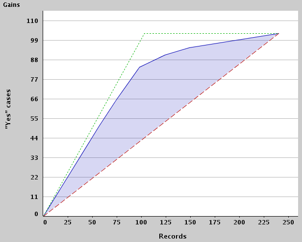
The blue line corresponds to ModelLiftGraph,
the green line to OptimumLiftGraph and
the red line to RandomLiftGraph.
Note that the latter two are not present in the example PMML, so the respective curves were derived from ModelLiftGraph.
Example:
Lift for a regression model predicting the field NUM_CLAIMS:
  ...
  <LiftData>
    <ModelLiftGraph>
      <LiftGraph>
        <XCoordinates>
          <Array n="7" type="int">5 12 18 23 31 41 52</Array>
        </XCoordinates>
        <YCoordinates>
          <Array n="7" type="real">80 70 48 40 53 64 66</Array>
        </YCoordinates>
        <BoundaryValues>
          <Array n="7" type="real">7.4261 7.1911 7.0731 6.9845 6.8072 6.6085 6.4999</Array>
        </BoundaryValues>
        <BoundaryMeanValues>
          <Array n="7" type="real">7.9327 7.6732 7.2982 6.9978 6.8734 6.7254 6.5373</Array>
        </BoundaryMeanValues>
      </LiftGraph>
    </ModelLiftGraph>
    <OptimumLiftGraph>
      <LiftGraph>
        <XCoordinates>
          <Array n="7" type="int">5 12 18 23 31 41 52</Array>
        </XCoordinates>
        <YCoordinates>
          <Array n="7" type="real">90 81 70 65 65 35 15</Array>
        </YCoordinates>
        <BoundaryValues>
          <Array n="7" type="real"> 8 7 6 5 4 3 2</Array>
        </BoundaryValues>
        <BoundaryMeanValues>
          <Array n="7" type="real"> 8.2872 7.8273 6.2362 5.7523 4.7895 3.4356 2.4563</Array>
        </BoundaryMeanValues>
      </LiftGraph>
    </OptimumLiftData>
  </LiftData>  ...
|
The lift data was built on a total of 52 records. The first 18 records
with the highest predicted values accumulate to 198, and the lower
limit for these is 7.0731. The third segment has 6 records accounts for
a sum of 48 with a mean value of 7.2982. The optimum model would have
predicted values that sum up to 70 in the same segment.
Here is the respective gains chart:
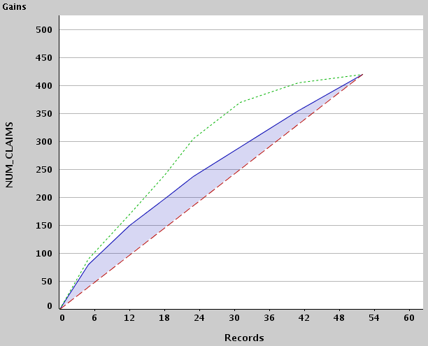
Again, the blue line corresponds to ModelLiftGraph,
the green line to OptimumLiftGraph and
the red line to RandomLiftGraph. Note that
OptimumLiftGraph is present in the sample PMML, while RandomLiftGraph had to be drieved
from ModelLiftGraph.
ROC (Receiver Operating Characteristic) Graphs are used in binary classification models.
The ROC curve is a graphical representation
of the sensitivity vs. (1 - specificity) for a binary classifier as its discrimination threshold varies. It
can also be represented by plotting the FPR (false positive rate) vs. the TPR (true positive rate).
  <xs:element name="ROC">
    <xs:complexType>
      <xs:sequence>
        <xs:element ref="Extension" minOccurs="0" maxOccurs="unbounded"/>
        <xs:element ref="ROCGraph"/>
      </xs:sequence>
      <xs:attribute name="positiveTargetFieldValue" type="xs:string"
                    use="required"/>
      <xs:attribute name="positiveTargetFieldDisplayValue" type="xs:string"/>
      <xs:attribute name="negativeTargetFieldValue" type="xs:string"/>
      <xs:attribute name="negativeTargetFieldDisplayValue" type="xs:string"/>
    </xs:complexType>
  </xs:element>
|
Attribute positiveTargetFieldValue in element ROC
gives the positive class label for which the ROC data is provided,
whereas attribute negativeTargetFieldValue in element ROC
gives the negative class label.
A normalized version, if applicable, can additionally be provided in
attribute positiveTargetFieldDisplayValue and negativeTargetFieldDisplayValue
(see attributes value and displayValue in DataDictionary).
  <xs:element name="ROCGraph">
    <xs:complexType>
      <xs:sequence>
        <xs:element ref="Extension" minOccurs="0" maxOccurs="unbounded"/>
        <xs:element ref="XCoordinates"/>
        <xs:element ref="YCoordinates"/>
        <xs:element ref="BoundaryValues" minOccurs="0"/>
      </xs:sequence>
    </xs:complexType>
  </xs:element>
|
In ROCGraph, FPR is provided in the XCoordinates, whereas TPR is provided in the YCoordinates.
FPR is defined as follows:
number of false positive records / (number of true negative records + number of false positive records)
TPR, on the other hand, is defined as follows:
number of true positive records / (number of true positive records + number of false negative records)
A boundary value represents a discrimination threshold or lower limit for the
respective score. That is, all records that are part of the segment
must have a value equal to or higher than the respective threshold in
BoundaryValues.
The point (0,0) in the graph is associated with the highest score and hence the highest limit;
it represents a binary classifier that predicts all cases to be negative.
The point (1,1) is associated with the lowest score and hence the lowest limit;
it corresponds to a classifier that predicts every case to be positive.
Example
The following sample code is for ROC data for a binary classification model:
  ...
  <ROC positiveTargetFieldValue="1" negativeTargetFieldValue="0">
    <ROCGraph>
      <XCoordinates>
        <Array type="real" n="6">0.13 0.2 0.28 0.56</Array>
      </XCoordinates>
      <YCoordinates>
        <Array type="real" n="6">0.54 0.75 0.86 0.93</Array>
      </YCoordinates>
      <BoundaryValues>
        <Array type="real" n="6">0.8 0.6 0.4 0.2</Array>
      </BoundaryValues>
    </ROCGraph>
  </GraphData>
  ...
|
Here is the respective ROC graph:
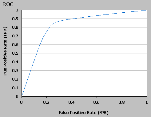
The ROC graph shows the tradeoff between the ability of a classifier to correctly identify positive records and the number of
negative records that are incorrectly classified.
The
ConfusionMatrix is used in classification models to give an overview of correct and incorrect classifications.
  <xs:element name="ConfusionMatrix">
    <xs:complexType>
      <xs:sequence>
        <xs:element ref="Extension" minOccurs="0" maxOccurs="unbounded"/>
        <xs:element ref="ClassLabels"/>
        <xs:element ref="Matrix"/>
      </xs:sequence>
    </xs:complexType>
  </xs:element>

  <xs:element name="ClassLabels">
    <xs:complexType>
      <xs:sequence>
        <xs:element ref="Extension" minOccurs="0" maxOccurs="unbounded"/>
        <xs:group ref="STRING-ARRAY"/>
      </xs:sequence>
    </xs:complexType>
  </xs:element>
|
ClassLabels specifies the class labels that the confusion matrix
refers to. New values in addition to the class labels of the initial
classification model are possible in a test result, if the test data
contains values that were not present in the training data.
The rows and columns of the Matrix refer to the sequence of the values as given in ClassLabels.
The rows in the matrix give the predicted class labels, while the
columns give the actual ones. The matrix must be square, and the number
of rows and columns must match the number of values in ClassLabels. Entries in the matrix must be of type integer.
Example
Here is an example for a classification model that predicts the domicile. The confusion matrix
|
suburban |
urban |
rural |
|---|
| suburban |
84 |
19 |
25 |
| urban |
14 |
123 |
17 |
| rural |
7 |
42 |
176 |
is represented by the following PMML code:
  ...
  <ConfusionMatrix>
    <ClassLabels>
      <Array type="string" n="3">suburban urban rural</Array>
    </ClassLabels>
    <Matrix>
      <Array type="int" n="3"> 84 19 25</Array>
      <Array type="int" n="3"> 14 123 17</Array>
      <Array type="int" n="3"> 7 42 176</Array>
    </Matrix>
  </ConfusionMatrix>
  ...
|
The confusion matrix tells that in 84 instances, the domicile was correctly predicted to be suburban.
In 17 instances, the domicile was predicted to be urban instead of rural. Likewise, in 7 instances
rural was predicted instead of suburban.
The
Correlations element is used to give correlations between fields used in a mining model.
  <xs:element name="Correlations">
    <xs:complexType>
      <xs:sequence>
        <xs:element ref="Extension" minOccurs="0" maxOccurs="unbounded"/>
        <xs:element ref="CorrelationFields"/>
        <xs:element ref="CorrelationValues"/>
        <xs:element ref="CorrelationMethods" minOccurs="0"/>
      </xs:sequence>
    </xs:complexType>
  </xs:element>

  <xs:element name="CorrelationFields">
    <xs:complexType>
      <xs:sequence>
        <xs:element ref="Extension" minOccurs="0" maxOccurs="unbounded"/>
        <xs:group ref="STRING-ARRAY"/>
      </xs:sequence>
    </xs:complexType>
  </xs:element>

  <xs:element name="CorrelationValues">
    <xs:complexType>
      <xs:sequence>
        <xs:element ref="Extension" minOccurs="0" maxOccurs="unbounded"/>
        <xs:element ref="Matrix"/>
      </xs:sequence>
    </xs:complexType>
  </xs:element>

  <xs:element name="CorrelationMethods">
    <xs:complexType>
      <xs:sequence>
        <xs:element ref="Extension" minOccurs="0" maxOccurs="unbounded"/>
        <xs:element ref="Matrix"/>
      </xs:sequence>
    </xs:complexType>
  </xs:element>
|
The CorrelationFields element specifies the field names that the correlations refer to.
These field names must match entries of MiningFields in the MiningSchema.
The CorrelationValues matrix holds the correlations in numeric form.
The rows and columns refer to the respective entries in CorrelationFields.
Valid entries must be in the range of [-1;1]. Values outside of this
range indicate that the correlation for the respective field combination is not available.
The CorrelationMethods element is optional and has string entries.
The entries correspond to the correlations given in CorrelationValues.
For each correlation provided in CorrelationValues, a respective entry must exist in the second one.
Valid values for the entries are:
- pearson: Pearson's correlation coefficient
- spearman: Spearman's rank correlation coefficient
- kendall: Kendall's τ
- contingencyTable: Contingency table
- chiSquare: Χ2 test
- cramer: Cramer's V
- fisher: Fisher's exact test
Note that some of these methods are distribution tests, since
especially for categorical fields, it is popular to use distribution
tests to express correlations. Entries that would refer to missing
entries in the
CorrelationValues must, if specified, still have one of these valid values.
If
CorrelationMethods is not present at all, defaults are
pearson for correlations
between numeric fields, and
contingencyTable for any other combination. Otherwise,
a corresponding entry for each entry in
CorrelationValues must be present.
Note that correlations between numeric and non-numeric fields are
usually done by defining buckets for the numeric field. These buckets are not covered here.
Note that both matrices must be symmetric.
Example
Here is an example correlation table:
  ...
  <Correlations>
    <CorrelationFields>
      <Array n="5" type="string"> "Age" "Angina" "Blood_Pressure" "Cholesterol" "Diseased" /Array>
    </CorrelationFields>
    <CorrelationValues>
      <Matrix kind="symmetric" nbRows="5" nbCols="5">
        <Array n="1" type="real"> 1</Array>
        <Array n="2" type="real"> 0.6207 1</Array>
        <Array n="3" type="real"> -0.2651 0.5793 1</Array>
        <Array n="4" type="real"> 0.2161 -99 0.1344 1</Array>
        <Array n="5" type="real"> 0.5649 0.5700 0.5257 -99 1</Array>
      </Matrix>
    </CorrelationValues>
    <CorrelationMethods>
      <Matrix kind="symmetric" nbRows="5" nbCols="5">
        <Array n="1" type="real"> pearson</Array>
        <Array n="2" type="real"> cramer cramer</Array>
        <Array n="3" type="real"> spearman cramer spearman</Array>
        <Array n="4" type="real"> fisher contingencyTable spearman spearman</Array>
        <Array n="5" type="real"> contingencyTable chiSquare chiSquare chiSquare chiSquare</Array>
      </Matrix>
    </CorrelationMethods>
  </Correlations>
  ...
|
For instance, according to this sample, the correlation between Age and Blood_Pressure is -0.2651
and was calculated using Spearman's rank correlation coefficient.
The correlation between Diseased and Cholesterol is not available.